Introduction
Note:
The analyses and results provided by FreeWeibull are based on statistical methods applied to the input data. The accuracy and applicability of the results depend on the quality and representativeness of the data.
This tool is intended for engineering evaluation and learning. Users are responsible for interpreting the results and applying appropriate engineering judgment.
FreeWeibull.com does not provide storage database for you to save your work. However, you can export it to your desktop in AssetStudio proprietary WTB file format, and import it for later use.
AssetStudio software suite includes FreeWeibull™, Weibull Toolbox™ and AeROS™.
FreeWeibull™ is a web-based application that consists of Life Data Analysis (LDA), Recurring Data Analysis (RDA) and Accelerated Life Testing (ALTA).
LDA is used to analyze the failure rate behavior of non-repairable items.
This analysis allows organizations to:
- Quantify the reliability performance at actionable item level.
- Justify improvement programs with statistical evidence.
- Optimize maintenance resources.
- Compare suppliers or designs based on statistical evidence.
- Verify failure trends of maintainable items/equipment.
- Project future costs due to failures.
- Others
Tip: FreeWeibull example files can be downloaded from: Help → Technical Support → Download Examples.
Life Data Analysis (LDA) Features:
- Supports all types of life data, including complete, right censored (suspended), left censored and interval censored, entered individually or in groups.
- Supports Probability-Time data type where user provides multiple probability-time pairs.
- Includes major lifetime distributions (Weibull, the Exponential, Lognormal and Normal).
- Includes a Reliability Test Tools for designing a reliability demonstration test plan.
- Includes a Simulation tool for visualizing the subtle relationship among sample size, confidence bounds and analysis methods.
- Provides a convenient Calculator to query commonly requested reliability results based on analysis together with required inputs.
- Provides results plots.
- Supports Bayesian-Weibull analysis for Weibull-2P, with a user-specified prior on the shape parameter β.
Recurring Data Analysis (RDA) Features
- Power Law or Crow-AMSAA (NHPP) models for repairable system analysis.
- Support Single System, Multiple Systems and Group Interval Data.
- Optimum overhaul time for a given repair cost and overhaul cost.
- Conditional reliability, MTBF or failure intensity for a given time.
- Expected number of failures for a given time.
- Time for a given conditional reliability, MTBF or failure intensity.
- Provides a convenient Calculator to query commonly requested reliability results based on analysis together with required inputs.
- Provide results plots.
Accelerated Life Test Analysis (ALTA) Features
- Supports complete, right censored (suspended) and interval censored data-type.
- Includes Weibull, Exponential and Lognormal distributions.
- Supports up to 3 simultaneous stresses Life-Stress Model.
- Supports Cumulative Damage Model allowing Time-Varying stress test.
- Calculator dialog for user to query common reliability question for a given analysis.
Further learning: For worked examples, see the Engineering Articles on AssetStudio.net. The directory covers reliability data analysis and digital twin simulation.
User Interface
Life Data Analysis (LDA) is active when the application is launched.
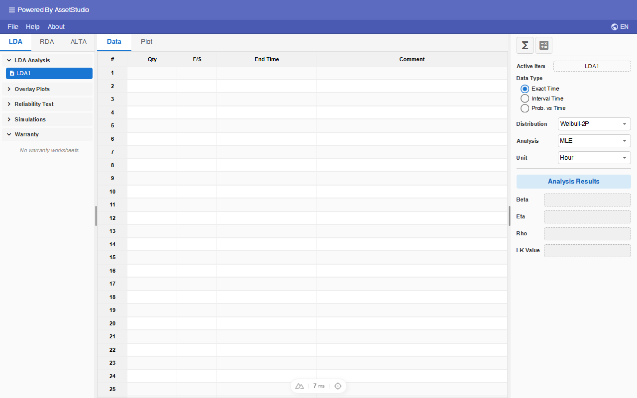
The Project Explorer area is categorized into Life Data Analysis (LDA), Recurring Data Analysis (RDA) and Accelerated Life Testing (ALTA).
LDA contains Worksheet, Overlay Plot, Reliability Test Design and Simulation list items. User can add more analysis items under each list.
ALTA contains Worksheet and Overlay Plot list items. Switch to the ALTA tab in the Project Explorer to add analyses.
The user interface for Data Entry and Plot area and Main Panel will change according the current active analysis. For standard Life Data Analysis worksheet, this area contains Data and Plot worksheets.
More descriptions of its functions in subsequence sections.
Life Data Analysis
Life Data Analysis Worksheet
To add additional LDA analysis, right-click on the worksheet list in the Explorer.
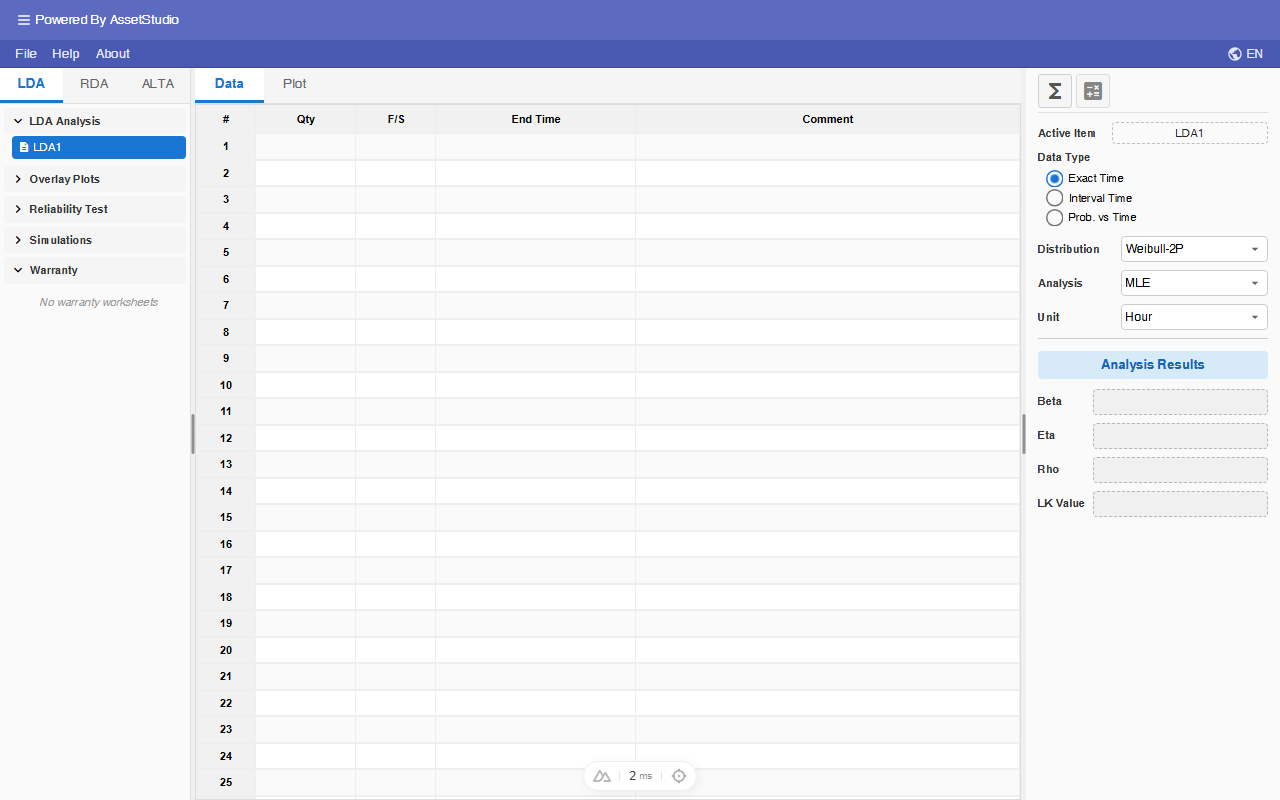
Data Entry
Life Data Analysis module supports 3 kinds of Data Type:
Exact Time Data Type
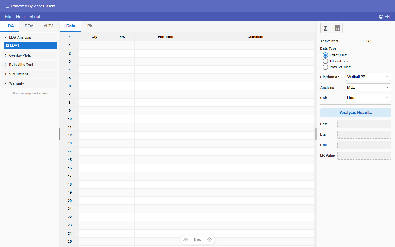
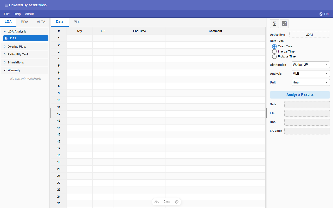
Assume a data set contains four exact failure times (hours) 20, 30, 40, 50 together with two suspensions at 60.
Enter the values under the in the column End Time. As you enter the data, Qty (Quantity) and F/S (Failure or Suspension) will be propagated with default values of '1' and 'F' respectively.
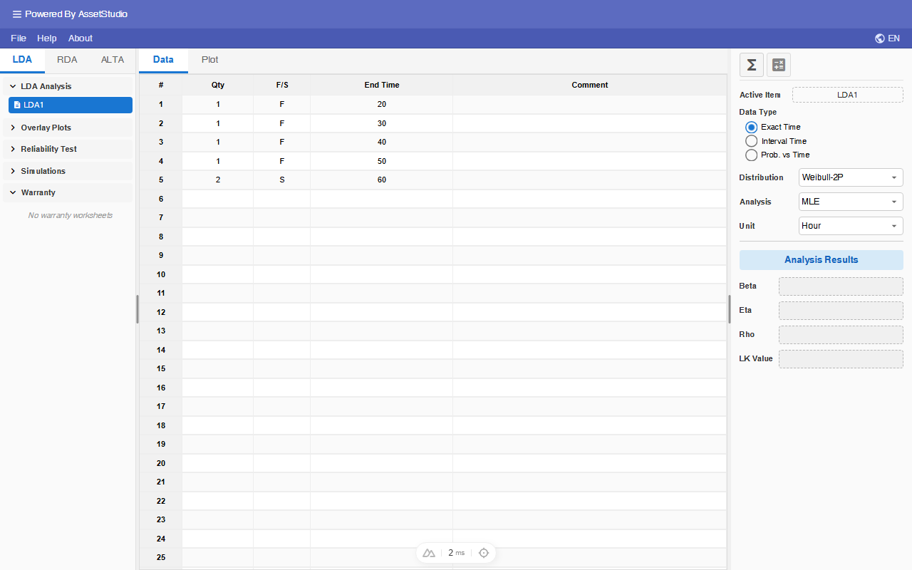
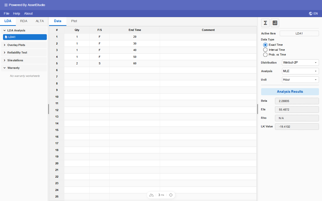
Since there are two suspensions at 60 hours, edit the corresponding Qty and F/S (at row 5) to '2' and 'S' as shown above. Click on the analysis icon .
Interval Time Data Type
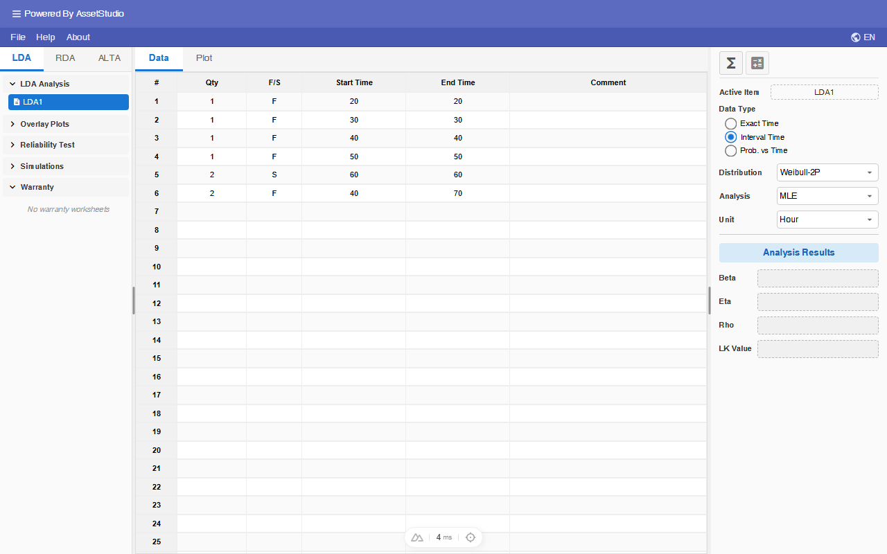
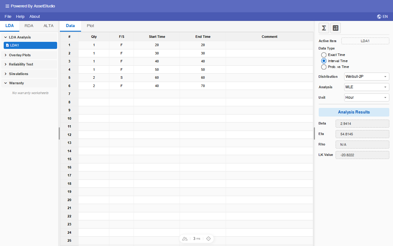
Assuming, in addition to the above exact time data, two items failed between 40 and 70 hours.
The current data type format (Exact Time) does not allow interval data. Switch to Interval Time data type by selecting 'Interval Time' of Data Type radio button.
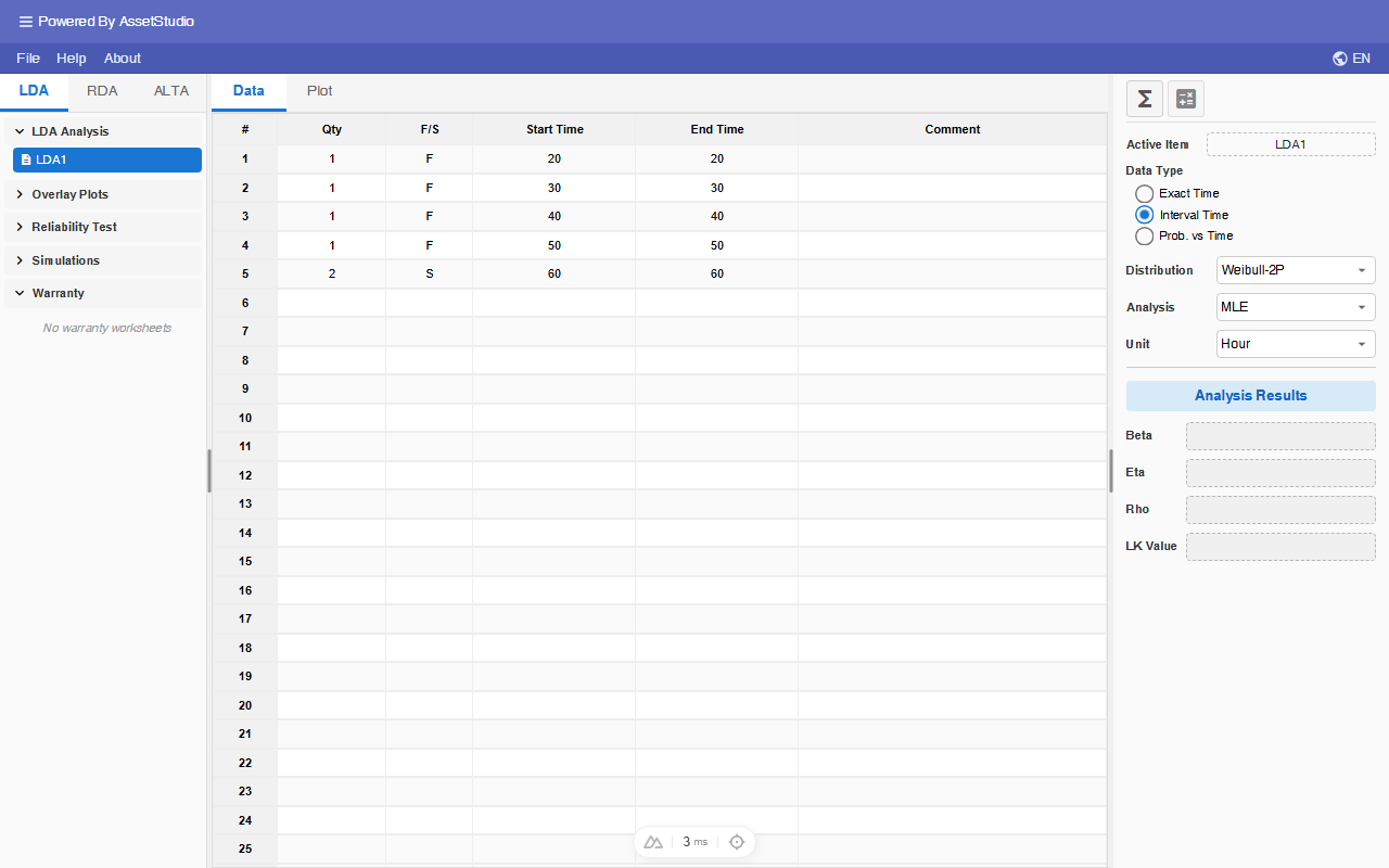
An additional column is added to accommodate Interval Time data type requirements. Note that the Interval Start Time column is filled with End Time data. The header text 'End Time' is changed to 'Interval End Time'.
Add the interval data (two items failed between 40 and 70 hours) as shown:
Probability-Time Data Type
Given that you know the probabilities of failure for a population at specific time points (for example, at 10, 30, and 50 days, the expected cumulative failure rates are 1%, 50%, and 90%, respectively), determine the distribution parameter values that best characterize the failure rate behavior of the population, based on your selected distribution. This analysis requires the use of the Probability-Time Data Type.
Add a new Worksheet (Right click on the worksheet list in the Explorer).
Select Probability vs Time radio button in Data Type of main panel, and enter the time-Probability pairs as shown, and click on the analysis icon .
Using a two-parameter Weibull distribution, the parameter values that best describe the failure rate behavior of the population are a shape parameter (β) of 3.45 and a scale parameter (η) of 36.76 days.
Note that
- For the Probability-Time data type, MLE, Bayesian-Weibull and confidence bounds calculations are not supported.
- RRY is the recommended fitting method for Probability vs. Time data.
- For two-parameter models, a minimum of two data points is required.
Calculate Parameters
Switch to LDA1 worksheet (or create a worksheet with the following data).
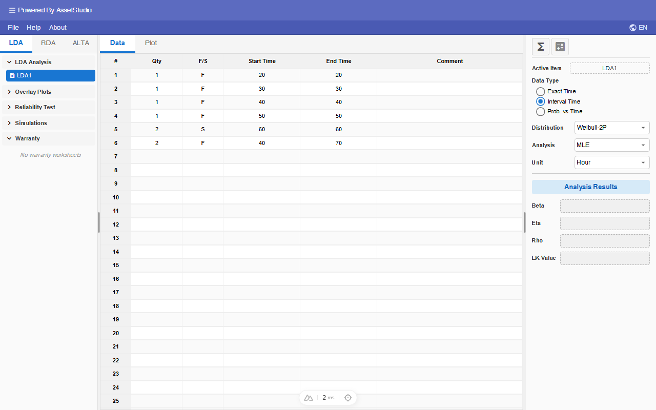
The default distribution is Weibull-2P. Other distributions available are Exponential, Normal and Lognormal and Weibull-1P.
Analysis Settings:
- Select Weibull-2P for Distribution.
- For analysis method, Maximum Likelihood Estimator (MLE), Rank Regression (RRX and RRY), and Bayesian-Weibull (Weibull-2P only) are available.
- As a rule of thumb, chose RRX for dataset with only complete data. If the dataset contains censored data, chose MLE.
- Select MLE for Analysis. Click on the Analysis icon to calculate the parameters.
The analysis fits the data to the distribution you chose, and the distribution parameters are shown in Analysis Results area.
Bayesian-Weibull
Bayesian-Weibull is available for Weibull-2P only. It places a prior on the shape parameter β and reports posterior point estimates for the Weibull parameters.
Select Weibull-2P for Distribution, then choose Bayesian in the Analysis dropdown. A Prior button appears next to Analysis.
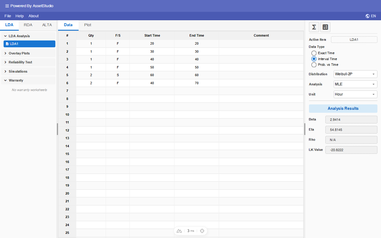
Click Prior to open the Bayesian-Weibull Prior dialog.
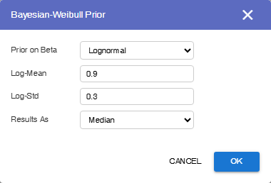
Prior settings:
- Prior Type (prior on β): Normal, Lognormal, Exponential or Uniform.
- Enter the prior parameters (for example Log-Mean and Log-Std for Lognormal; Mean and Std. Dev. for Normal; Lambda for Exponential; Min Beta and Max Beta for Uniform).
- Results As: Median or Mean (how the posterior point estimates are reported).
Click OK, then click the Analysis icon to calculate. Plot confidence bounds switch to the Bayesian method; Fisher Matrix and Likelihood Ratio are disabled.
Note that
- Bayesian-Weibull is not available for Probability-Time data.
- Contour plot is not available for Bayesian-Weibull worksheets.
- If an overlay plot includes only Bayesian-Weibull worksheets, overlay confidence bounds use the Bayesian method.
Plots
Click on the Plot tab at the top of worksheet area. The default plot type is the Unreliability plot. You can access the other plots through Plot Type dropdown list.
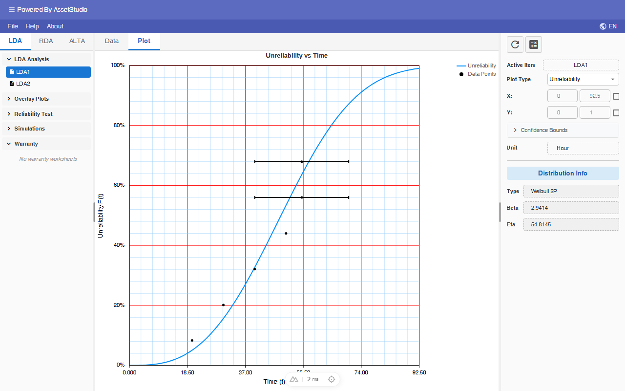
Available plots are:
- Model Probability
- Reliability vs Time
- Unreliability vs Time (Cumulative Density Function)
- PDF (Probability Density Function)
- Failure Rate vs Time
- Contour Plot (available for 2-parameter distributions)
Confident Bound on plots
- Switch Plot Type to Probability (and click on to refresh the plot).
- Click on Confidence Bounds button.
- Select Two-Sided 90% level.
- Select Bound On Y-Axis. Assuming you want to read Reliability (Y-Axis) given time. If you want to read the time (X-Axis) for given Reliability, then you should choose Bound On X-Axis.
- Click on the re-calculate icon .
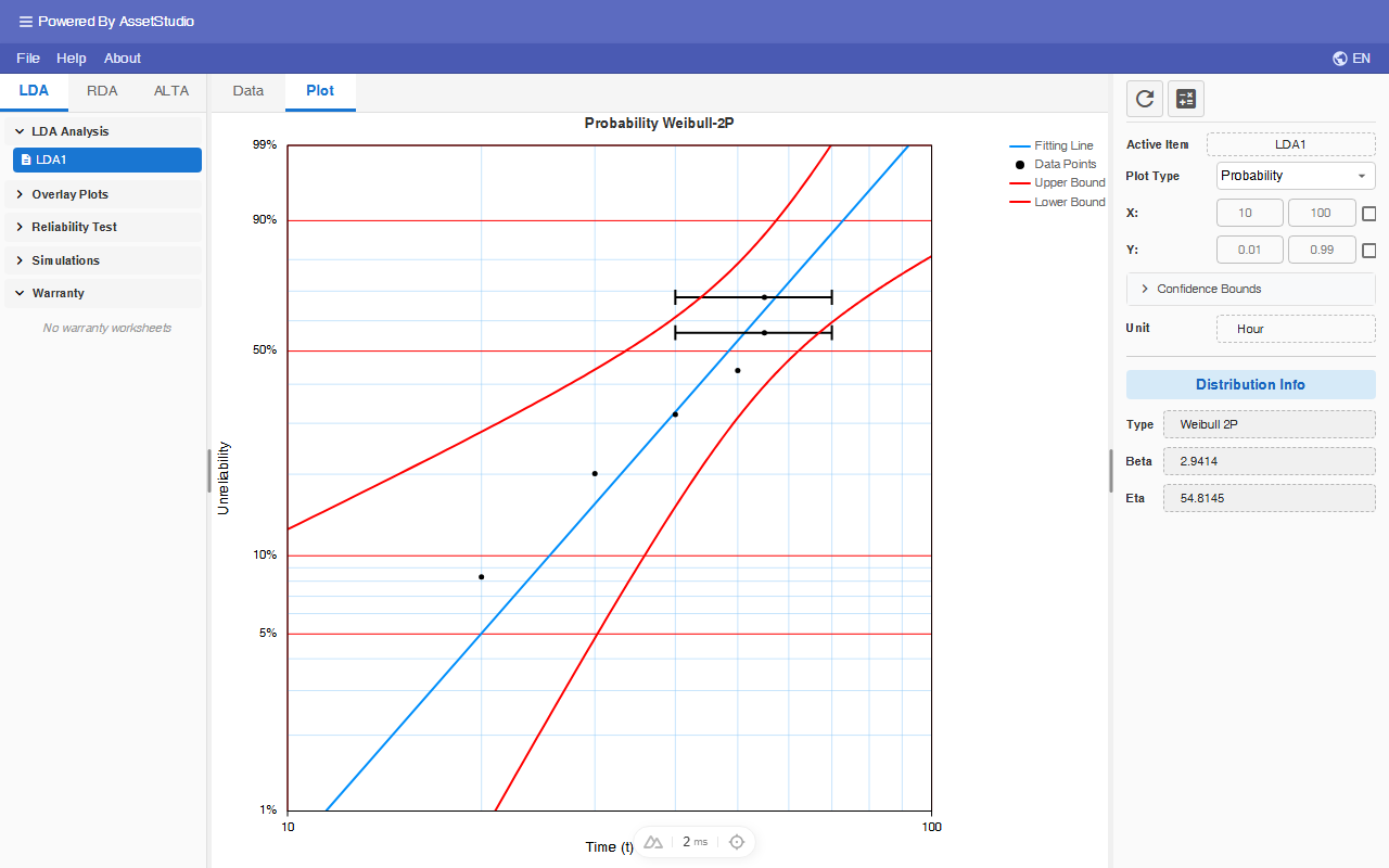
You can Left-Click on the plot area to read the Time-Probability coordinate.
For a Bayesian-Weibull analysis, plot confidence bounds use the Bayesian method; Fisher Matrix and Likelihood Ratio are disabled.
Calculator
Click on the Calculator icon at the top of main panel.
This tool allows you to query commonly requested reliability results based on your analysis together with required inputs.
| Matrix | Results | Required Input |
|---|---|---|
| Reliability | Probability of Success at mission time, T | Time T |
| Unreliability | Probability of Failure at mission time, T | Time T |
| Conditional Reliability | Probability of Success for a mission time t, given start time (current age) T. | Start Time T, and Additional Time t |
| Conditional Unreliability | Probability of Failure for a mission time t, given start time (current age) T. | Start Time T, and Additional Time t |
| BX Life | The time by which X% of the population fails. | Percentage failed BX (%) |
| Warranty Life | The time by which a given fraction of the population still survives. | Reliability |
| Failure Rate | Failure rate at mission time T. | Time T |
| Mean Life | Average life of the population. | None |
| Useful Life | Remaining Average life, given the current age, T, of the population. | Start Time T |
| Optimum Replacement Time | The optimum Preventive Maintenance Interval. | Corrective maintenance and Preventive maintenance costs |
Select Unreliability radio button and enter Time = 30 as shown.
Set the confidence bounds to FM/90/2S (Fisher Matrix, 90%, 2-sided). Click on Calculate button.
When the worksheet is a Bayesian-Weibull analysis, the calculator confidence-bound method is Bayesian (Fisher Matrix and Likelihood Ratio are not used).
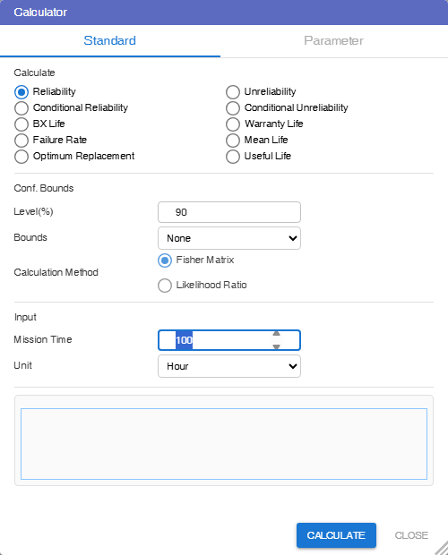
Compare the results with that obtained from probability plot earlier.
Select Optimum Replacement radio button to calculate the optimum preventive maintenance interval.
Assume the Corrective Maintenance (CM) and Preventive Maintenance (PM) costs are $1000 and $500 respectively.
Note that for Optimum Replacement calculation, the following conditions must be satisfied:
- CM cost must be greater than PM cost.
- Failure rate must be increasing.
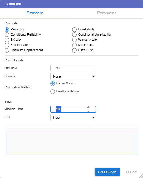
Interpretation: If run-to-failure (or condition monitoring) is not an option, it costs you least to replace at every 45 hours of usage.
The Calculator will return NaN (non-a-number) code if Optimum Replacement interval does not exist.
Overlay Plot
You can compare the plots across different standard worksheets using Overlay Plot.
The following example demonstrates an Overlay Plot of two Probability-Weibull curves of the same data set analyzed using MLE and RRX respectively. The data set is as follow, 20, 30, 40, and 50. Unit is in hour.
- Create 2 standard worksheets, rename the worksheets accordingly, and enter the date to both worksheets.
- Analyze one with MLE while the other with RRX.
- Right click on Overlay Plot list to add an Overlay Plot.
Select Data Source dialog appears. Select both worksheets as shown:
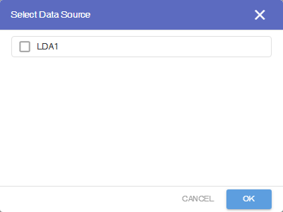
Click OK.
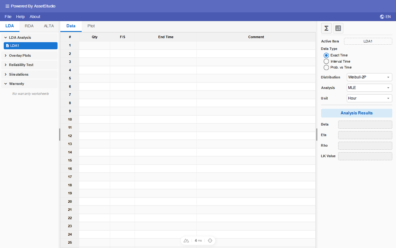
You can also change to other Plot Types (Reliability, Unreliability, PDF, Failure Rate or Contour plot).
If every selected overlay worksheet was analyzed with Bayesian-Weibull, the confidence-bound calculation method switches to Bayesian (Fisher Matrix and Likelihood Ratio are disabled). Contour plot is not available for Bayesian-Weibull worksheets.
Random Number Generator
You can generate a set of random numbers based on selected distributions.
Right click on any existing LDA worksheet and a pop-up menu appears. Select Random Data item.
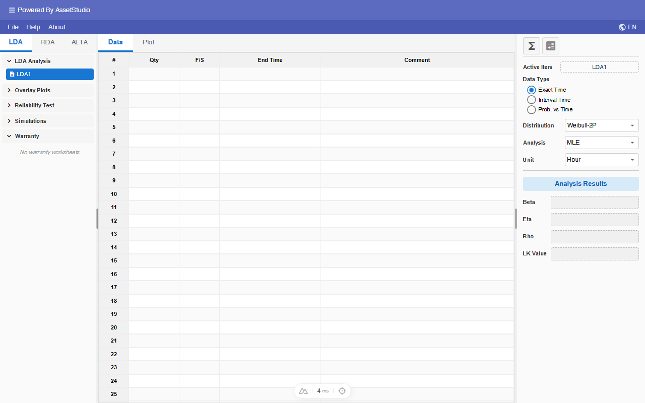
Random Number Generator dialog appears.
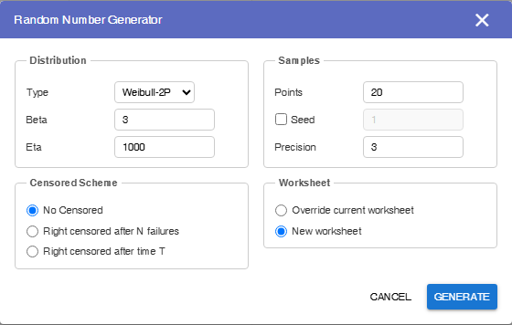
You can set the Distribution type, Sample generation options and Censoring scheme. You have the option to place the data set on the current worksheet or a new worksheet.
Click Generate button to create the data set.
Reliability Test
This tool is to help test engineer to design a reliability test plan so as to demonstrate that a product has met a goal of a certain reliability at a given time with a specific confidence.
User must supply
- The reliability target to be demonstrated.
- Number of failure(s) to be observed.
- The assumed distribution (Weibull, Normal, Lognormal and Exponential).
- Depending on the assumed distribution, further assumption on the parameter value is required:
- For Weibull distribution, β value is to be provided.
- For Normal distribution, μ (standard deviation) value is to be provided.
- For Lognormal distribution, Log-μ (Log-standard deviation) value is to be provided.
If user provide the available test time, the tool solves for the required number of test units in order to meet the reliability target.
If user provide the available test units, the tool solves for the required test time in order to meet the reliability target.
To add a Reliability Test analysis, right click on the Reliability Test tool in Explorer.
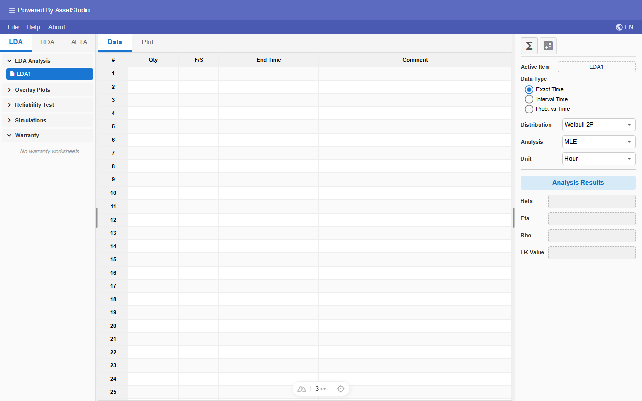
'Test1' analysis item is added under Reliability Test list. Click on 'Test1' item icon and Reliability Test design tool appears.
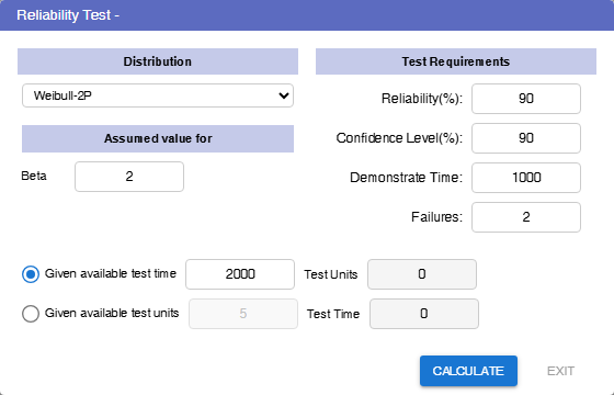
In the following example, the test engineer wishes to design a test to demonstrate a reliability of 90% at 500 hours with a 90% confidence, no failure allowed during the test. Weibull distribution with beta = 3 is assumed.
The available time to execute the test is 600 hours.
Enter the required specifications as shown a click Calculate button.
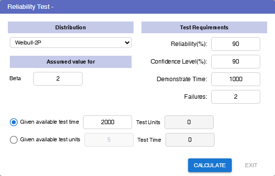
13 units are required to operate for 600 hours without failure to demonstrate that R(500) > 0.9 with 90% confidence level.
Simulation
This tool allows user to define the distribution, the sampling size, censoring scheme and the number of datasets to generate. The analysis method (MLE, RRX or RRY) is applied to estimate distribution parameters of each dataset, and Probability plot of each dataset is superimposed on the same graph.
This simulation tool allows user to,
- Visualize the biasing effect of sample sizes and censoring schemes on analysis methods (MLE and Regression)
- Visualize how sample sizes and censoring schemes affect confidence bounds,
- Provide an intuitive meaning of confidence bounds,
- Provide a way to decide the sample size for reliability demonstration tests.
To add a Simulation worksheet, right click on the Simulation tool in Explorer, and click on Add Simulation popup menu.
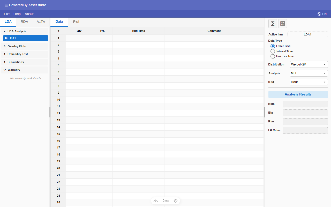
Simulation setting dialog appears.
In the default settings, the distribution is Weibull (3, 1000). It will generate 500 datasets of 10 uncensored data points each, and RRX analysis method is applied.
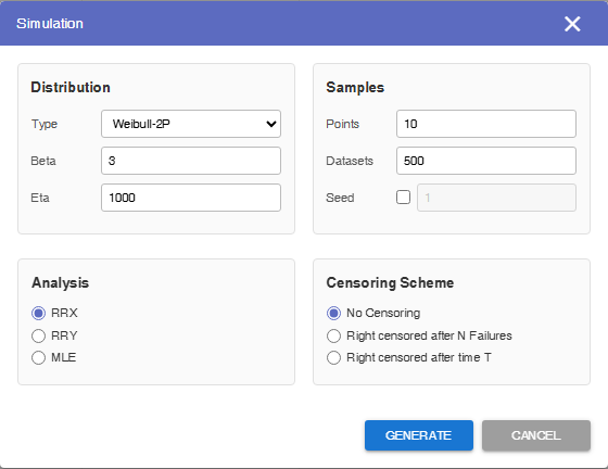
Set Seed to 1 and click on Generate data button.
500 datasets are generated and fitted to Weibull distribution. The parameters values of each dataset are listed in the worksheet. Click on the Plot tab.
The graph shows the Probability Weibull plots of all the corresponding 500 datasets. The 'Original Line' is plotted in black. The confidence bounds are plotted at 80% level (both one-sided).
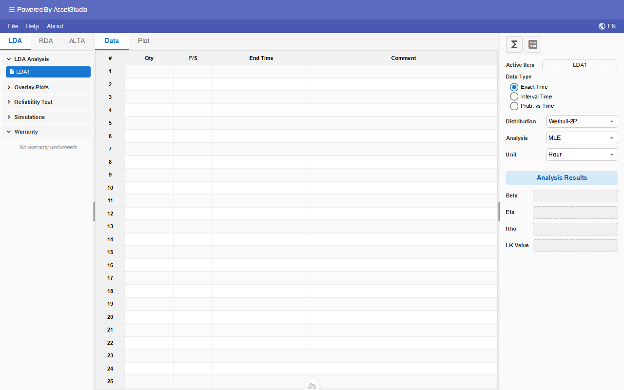
Consider a reliability test produces 10 exact Time-To-Failure points. It fits to Weibull distribution with β and η equal to 3 and 1000 hours respectively.
The B(10) life is η(ln 11−0.1)1β = 472 hours (@50% CL One-Sided)
Suppose the requirement is to demonstrate B(10) life of 300 hours with 80% CL.
Does this test demonstrate that the requirement is met? (Yes, see plot below)
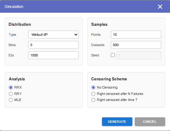
Warranty Analysis
The purpose of this warranty analysis tool is to forecast the failures in the future, given the historical sales quantity and those observed returns.
To add a warranty worksheet, right click on the Warranty tool in Explorer, and click on Add LDA Warranty popup menu.
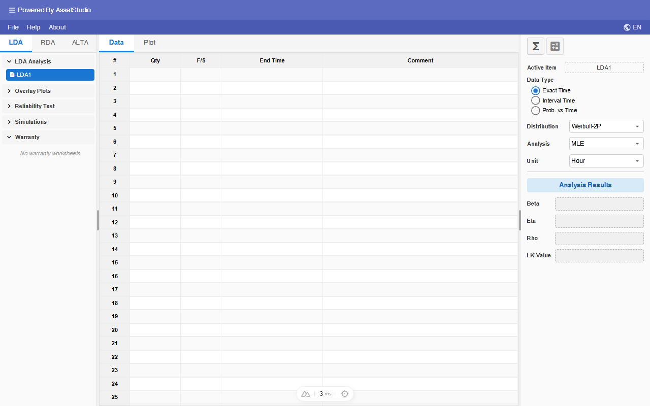
Click on Warranty1 item.
The following example can be found in: UserGuide→UserGuideWarranty.wtb
Import UserGuideWarranty.wtb (File → Import)
The data warranty analysis is available in the MS Excel file UerGuideData.xlsx in the UserGuide folder.
This worksheet contains Sales, Returns, Data, Plot, Future Sales and Forecast tabs.
- Sales tab – User enters the shipment quantities and its corresponding calendar dates (Date In-Service).
- Returns tab – User enters the returns' dates, and its corresponding Data In-Service.
- Data tab – It contains the Time-to-Failures dataset which is derived from Sales and Returns information entered by the user. This dataset is used for calculating the failure distribution of the population.
- Plot tab – It is for displaying reliability related plots.
- Future Sales tab – User provides future sales here.
- Forecast tab – Based on sales (include future sales) and returns, it calculates and displays failure forecast.
In the Sales tab, there were 6 shipments. In the first row, for example, 200 units were shipped on the 1-Jan-2026.
The Returns tab shows the returned units date with the corresponding return data and 'Date In-Service'. The 'Date In-Service' is used to identify with shipment it belongs to.
Click on the analysis icon to calculate the distribution parameters based on user analysis settings.
The Data tab will now contain the Time-to-Failures dataset which is derived from Sales and Returns information provided.
Assuming we want to forecast the returns in the next 6 months, starting from 2nd July 2026, for the products already in service, plus the following future sales:
Click on the forecast icon .
In the Forecast dialog, enter the followings:
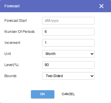
Click OK button.
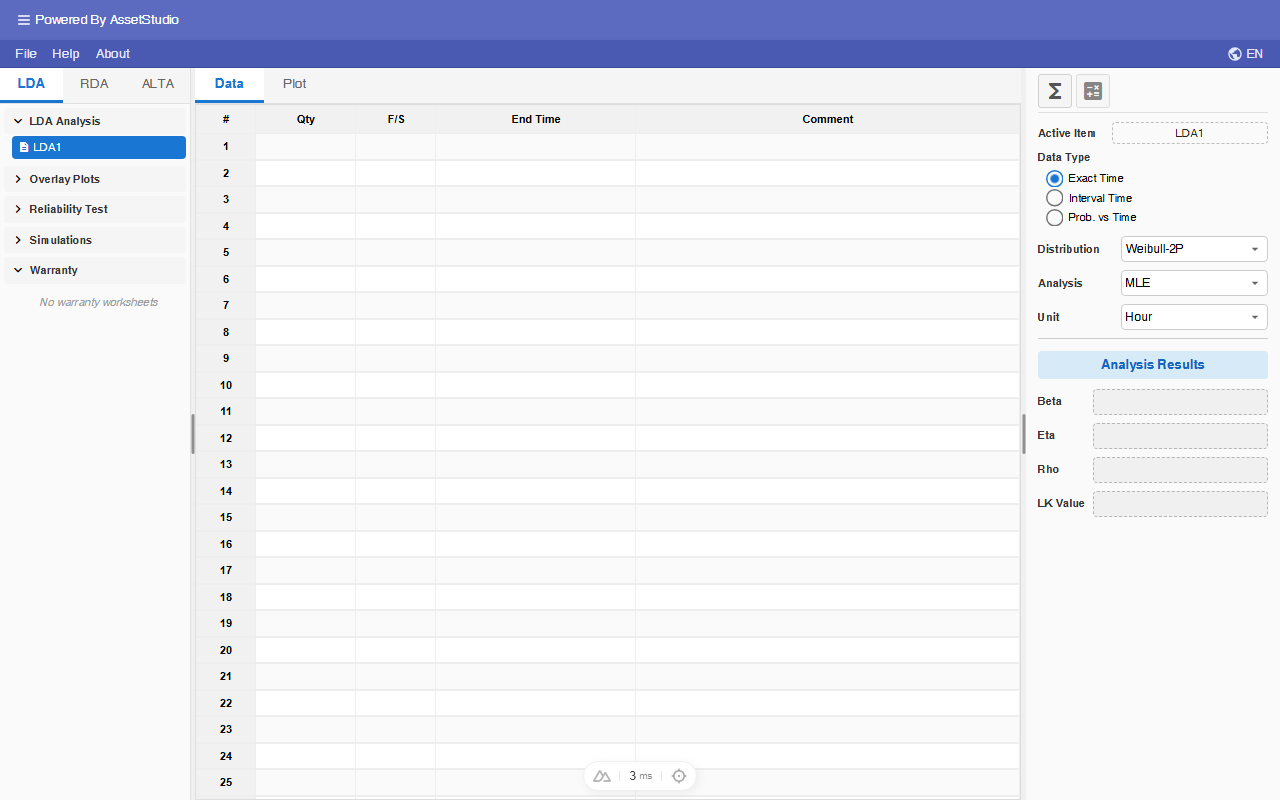
The Forecast tab displays the expected returns over a total of six periods. The first column represents the returns from the latest return date to the forecast start date, while the remaining five columns correspond to subsequent one-month periods.
Note that the Forecast Start date must be larger than the latest return date.
Recurring Data Analysis
Recurring Data Analysis Worksheet
Life Data Analysis is active when the application is launched. You can switch it to Recurring Data Analysis (RDA) from Explorer panel. Click on the RDA tab in Explorer panel.
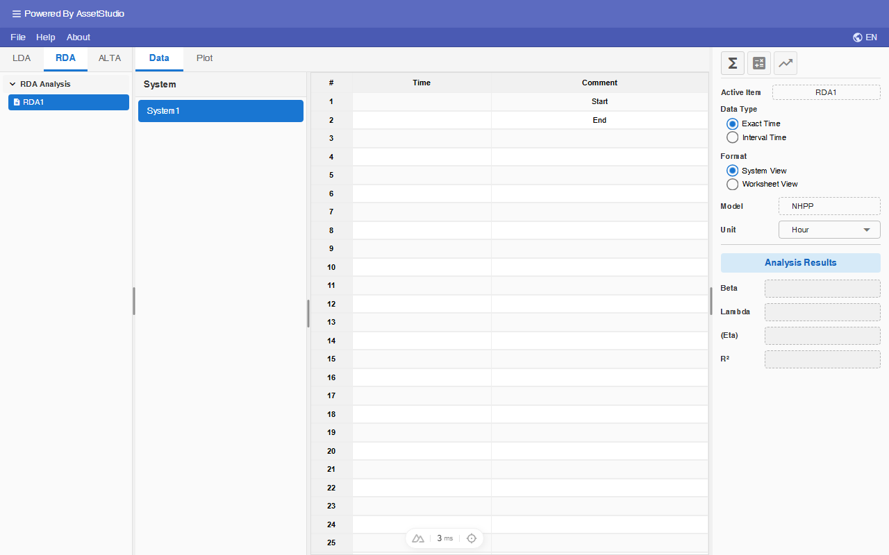
You can add additional RDA (or delete) analysis by right click on the RDA analysis tree list in the Explorer.
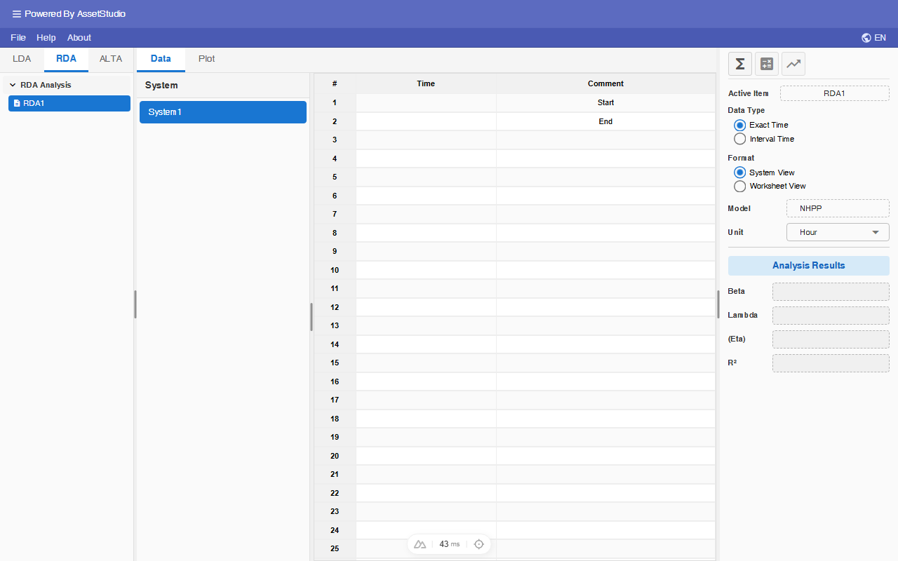
To add new system, right click on the System panel client area.
Data Entry
Recurring Data Analysis module supports 2 kinds of Data Type:
Exact Time Data Type
Followings are the cumulative failure records (in days) of 3 pumps working under similar stress condition.
The following example can be found in: Examples→UserGuide→UserGuideRDA.wtb
Enter the above data into RDA worksheet as described below.
Rename System1 to Pump1, and enter Time to Event data as shown.
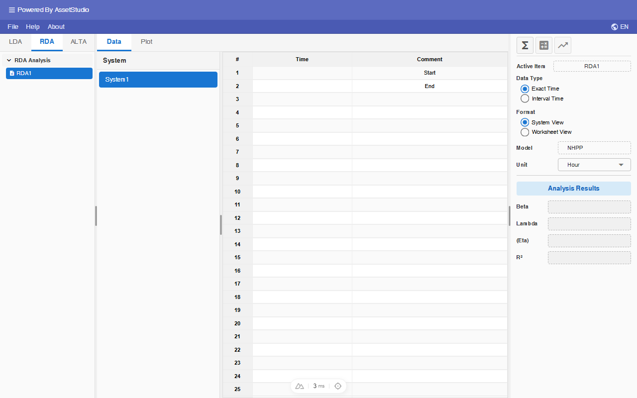
Note that the time Unit is set to Day.
Enter the data for Pump2 and Pump3.
Click on the Analysis icon to calculate the NHPP model parameters.
Select Worksheet format from the main panel. The Worksheet Format presents the entire dataset in one single worksheet.
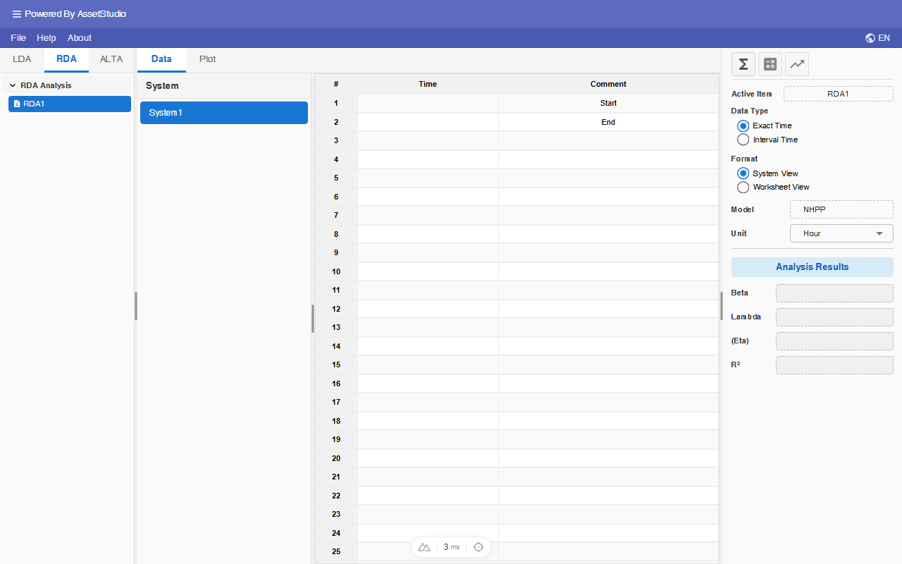
This format makes it easier to import and export data to and from Excel.
Interval Time Data Type
Consider the following group failure data of two repairable machines, M1 and M2, measured in hours.
System M1
| Failed Qty | Interval | |
|---|---|---|
| Start | End | |
| 1 | 0 | 200 |
| 2 | 200 | 400 |
| 3 | 400 | 600 |
| 4 | 600 | 750 |
System M2
| Failed Qty | Interval | |
|---|---|---|
| Start | End | |
| 1 | 0 | 400 |
| 2 | 400 | 600 |
| 3 | 600 | 900 |
Add a new RDA worksheet from the Worksheets tree in Explorer panel.
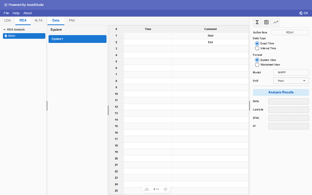
Select Interval Time data type from the main panel. For Interval Time data type, failure data can only be entered in the Worksheet format.
Enter the group failure data of machine M1 and M2 into the worksheet as shown. Click on the Analysis icon to calculate the NHPP model parameters.
Calculate the Parameters
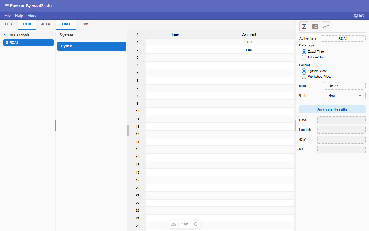
Switch back to 'RDA1' worksheet and click on the Analysis icon .
The calculated parameters will appear in the Analysis Results area.
The NHPP model with Power Law can also be expressed with Time-To-First-Failure Weibull distribution, where eta, η = (1λ)1β
Rho is the co-relation coefficient for the cumulative failure vs time plot in Log-Log scale. It indicates how well the dataset forms a straight line. A value of 1 means the dataset forms a perfect straight line.
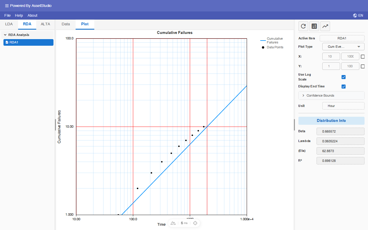
The above is cumulative failure vs time plot in Log-Log scale.
Plots
Click on the Plot tab at the bottom-left of data-grid worksheet. The default plot is the Probability Plot. You can access the other plots through Plot Type dropdown list.
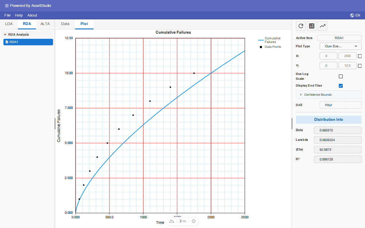
Available plots are:
- Cumulative Failures vs Time
- MTBF vs Time
- Failure Intensity vs Time
By default, plots are displayed in linear scale. Select Use Log Scale checkbox for Log-Log scale.
Confident Bound on plots
Click on Confidence Bounds button in the main panel and set 90% Two-Sided bound.
Click on refresh icon .
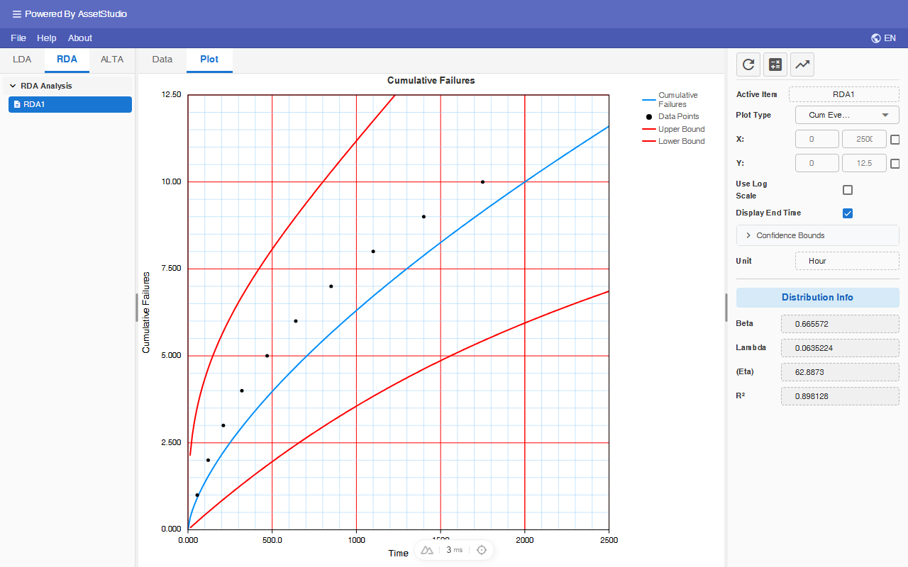
For a new pump, what is the expected number of failures by 600 days of age, with 90% two-sided confidence bounds?
* Lower bound = 1.6,
* Upper bound = 4.4
Calculator
Click on the Calculator icon at the top of main panel.
This tool allows you to query commonly requested reliability results based on your analysis together with required inputs.
| Matrix | Results | Required Input |
|---|---|---|
| Reliability | Probability of Success for a mission time t, given current age T. | Current Age T, and Mission Time t |
| Number of Failures | Expected cumulative number of failures for a mission time t, given current age T. | Current Age T, and Mission Time t |
| Inst. MTBF | Instantaneous MTBF at mission time T. | Mission Time T |
| Inst. Failure Intensity | Instantaneous Failure Intensity at mission time T. | Mission Time T |
| Mission Time (Age, R) | The mission time for a required reliability and current age T. | Current age T, and Reliability R |
| Age (Mission Time, R) | Find the Age such that a mission time T can be achieved for a required reliability | Mission Time T, and Reliability R |
| Optimum Overhaul | Find the optimum overhaul time | Repair cost, and Overhaul cost |
Select Number of Failures radio button
Set the Confidence Bound: 90%/Two-Sided
Set the required input Current Age and Mission Time to 0 and 600 days respectively.
Click on Calculate button.
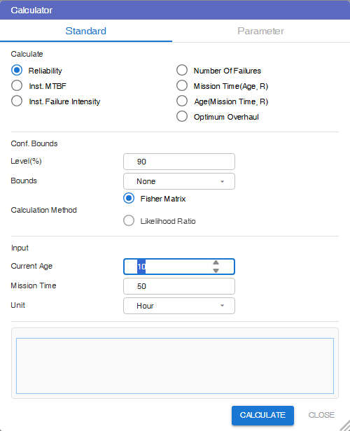
Compare the results with that obtained from Cumulative Failures plot in previous section.
Given that the repair cost and overhaul cost are $1000 and $5000 respectively, determine the optimum overhaul time.
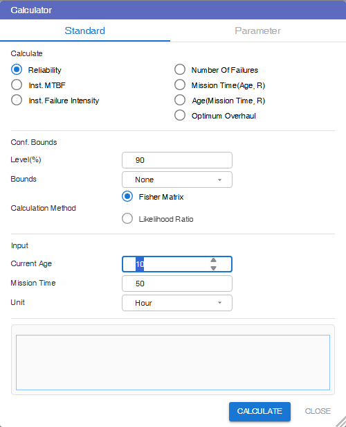
Note that Optimum Overhaul exists provided that the item has an increasing failure intensity, and the Overhaul cost is significantly more expensive than Repair cost.
Failure Forecast
This tool is used to forecast the expected number of failures in the future for a fleet of repairable items.
The following demonstrations is based on RDA1 example (Pump dataset).
We assume that all the 3 pumps operate round the clock.
Let's also consider you as the pump manufacturer. You have entered into a 30-month contract to maintain the fleet of pumps. Your objective is to predict the anticipated number of failures per quarter over the upcoming 30 months in order to effectively plan maintenance. Additionally, assume you offer a 42-month warranty for each pump, meaning you are not responsible for pumps older than 42 months.
From the Data worksheet view click on the Forecast icon at the top of main panel.
In the Failure Forecast dialog, enter the following settings:
- Interval – 3 Months
- Num. of Intervals – 10
- Warranty Period – 42 Months
Click on Re-calculate button. The dialog displays the projected failures for each quarter over 30 months (10 intervals), as shown:
The Total row (4th row) indicates the total projected failures for each quarter.
Pump1 has a current age of 1095 days (36 months), and the warranty covers 42 months. This implies that the warranty will conclude after an additional 6 months of operation. Consequently, once this additional 6-month period elapses, maintenance responsibility will no longer rest with you, and the estimated number of failures is anticipated to be zero from that point onward.
The Usage Rate is set to 100% because the pumps operate round the clock. If, for example, a pump only operates 8 hours a day, its Usage Rate would have been 33.33%.
The Check-box column (1st column) is for user to select the systems to be removed.
Accelerated Life Test Analysis
The main objective of Life Data Analysis (LDA), in the manufacturing environment, is to determine the Probability Density Function (PDF) of a population of items. Quantitative accelerated life testing is used to achieve the same objective faster, by applying appropriate stress (or stresses) that can cause the items to fail faster.
In order to complete the test faster, experiments are conducted at higher stress levels. Use-level PDF is obtained by extrapolating from the high stress level PDFs along a Life-Stress-Relationship model.
Accelerated Life Test Analysis (ALTA) Worksheet
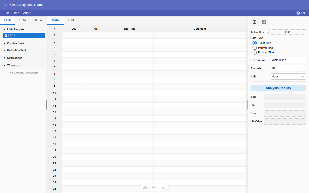
To access the Accelerated Life Test Analysis (ALTA) Worksheet, click on the ALTA tab in the Explorer panel.
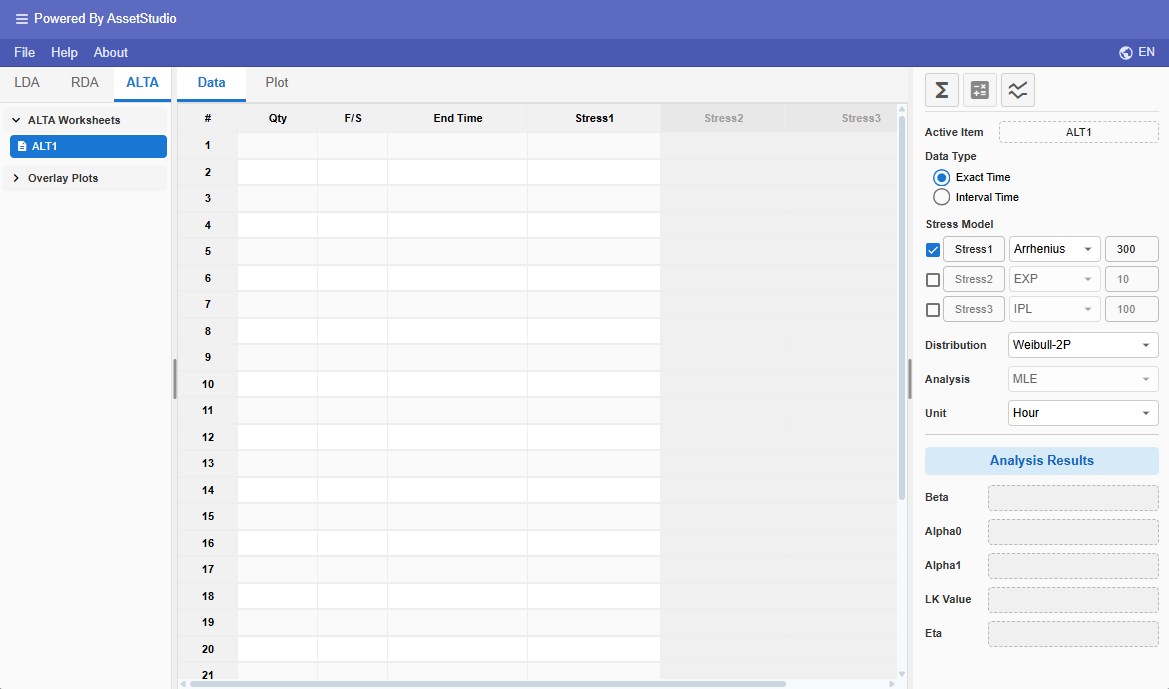
The Worksheet Area is the same as that of LDA, except that it contains stress columns. FreeWeibull ALTA supports up to 3 simultaneous stresses.
Data Entry
ALTA supports two data types: Exact Time and Interval Time. Each row has life-time columns (quantity, F/S, time) plus one or more stress columns.
Exact Time Data Type
In Exact Time mode, each row records a failure or suspension at a known time. Enter the quantity in Qty, the type (F for failure or S for suspension) in F/S, and the time in the Time column.
For each enabled stress column, enter the constant stress level that the test units were subjected to at that time point. See Entering Stress for details on stress columns.
Example 1: Dataset with Single Stress
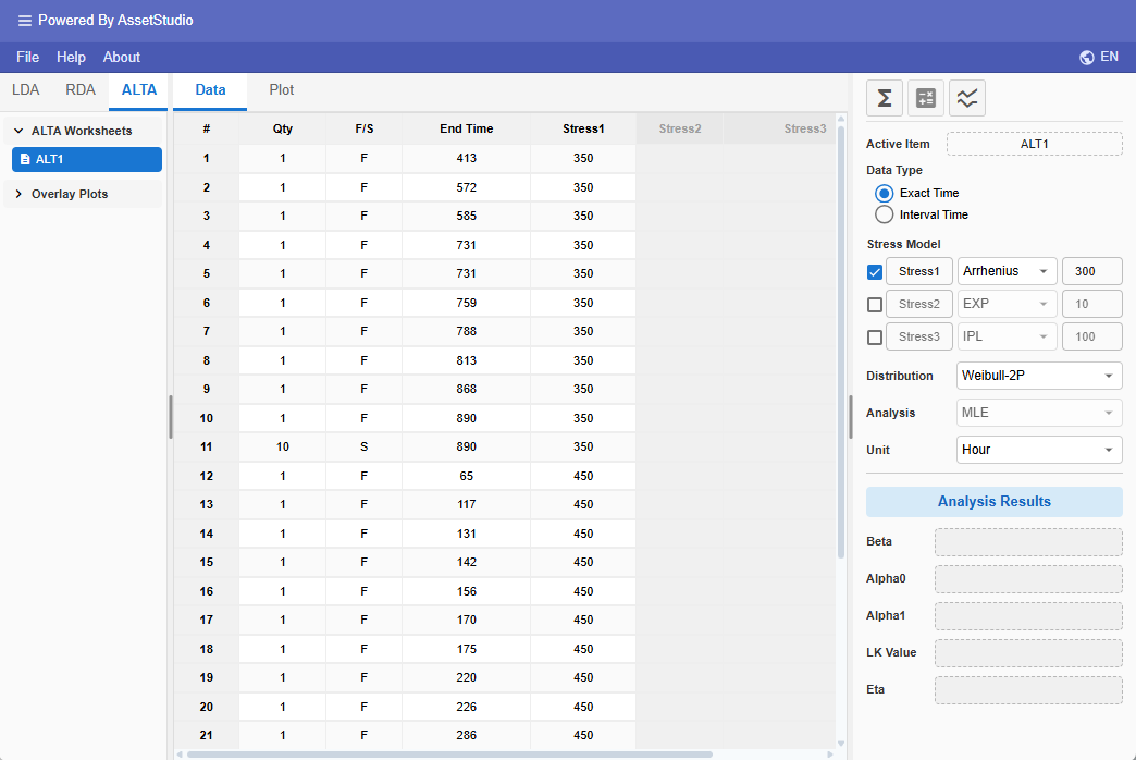
An accelerated life test was conducted with temperature as the stress. 20 units were tested at 350-degree Kelvin. This test was censored after the 10th failure. Another 10 units were tested at 450-degree Kelvin.
Temperature = 350K
| Qty | Status | TTE/hour |
|---|---|---|
| 1 | F | 413 |
| 1 | F | 572 |
| 1 | F | 585 |
| 1 | F | 731 |
| 1 | F | 731 |
| 1 | F | 759 |
| 1 | F | 788 |
| 1 | F | 813 |
| 1 | F | 868 |
| 1 | F | 890 |
| 10 | S | 890 |
Temperature = 450K
| Qty | Status | TTE/hour |
|---|---|---|
| 1 | F | 65 |
| 1 | F | 117 |
| 1 | F | 131 |
| 1 | F | 142 |
| 1 | F | 156 |
| 1 | F | 170 |
| 1 | F | 175 |
| 1 | F | 220 |
| 1 | F | 226 |
| 1 | F | 286 |
Enter the data into the ALTA worksheet as shown. The Life-Stress Model and underlying distribution are set to Arrhenius and Weibull respectively.
Interval Time Data Type
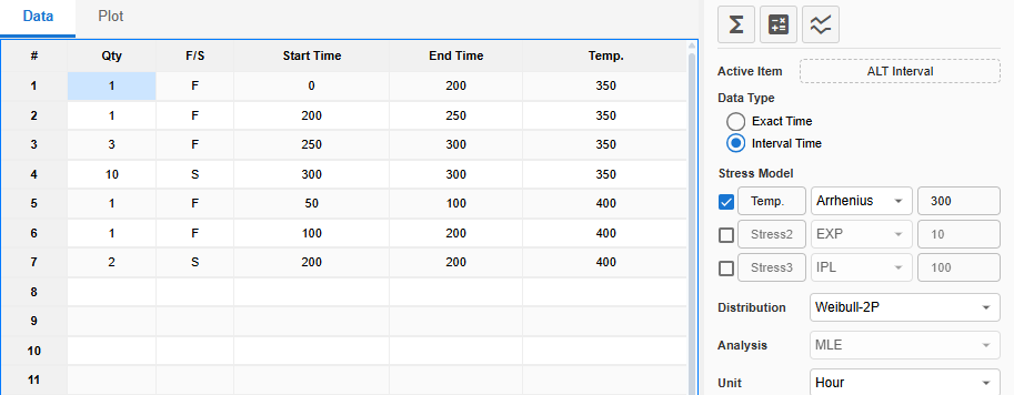
In Interval Time mode, failures are known to have occurred within a time interval rather than at an exact time. Enter the interval bounds in the Start Time and End Time columns.
Suspensions in Interval Time mode are recorded with the last known alive time in Start Time and a blank or large value in End Time. Stress columns work the same as Exact Time mode.
The following is an example of a data set with complete, suspended, interval and left censored data.
Entering Stress
Each stress column has a combo box. Select (constant) to enter a numeric stress level directly in the cell, or choose a named stress profile for time-varying stress.
When (constant) is selected, type the numeric stress value (e.g., temperature in °C, voltage in V) directly in the cell. This is the simplest way to enter data for a constant-stress accelerated test.
When a named profile is selected, the stress level varies over time according to that profile's definition. Use the Stress Profiles manager to create and edit profiles before assigning them to data rows.
Stress Profiles
The following section describes how to create a time-varying stress profile.
Click the Stress Profiles toolbar icon (next to Calculator) to open the manager.
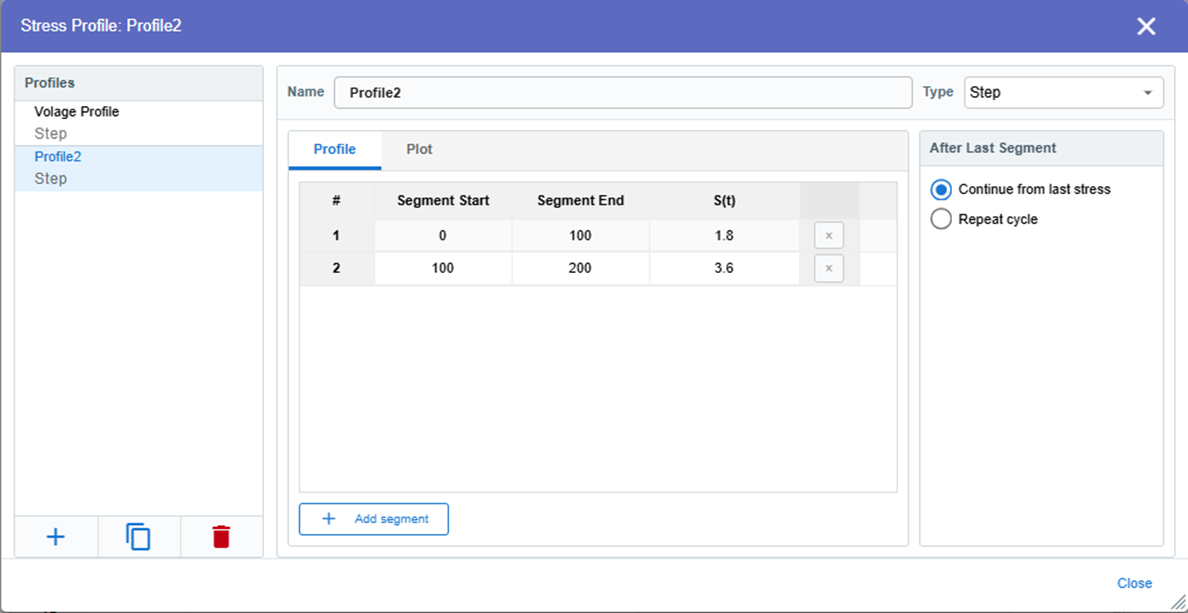
Add named profiles on the left. For the selected profile, choose a type and edit the segment grid. Available types:
- Step – successive dwells at constant stress.
- Linear Ramp – stress changes linearly from a start level to an end level.
- Trapezoid Cycle – ramp up, high dwell, ramp down, low dwell (optionally repeated).
- Piecewise Linear – a sequence of time-stress knots.
After Last Segment: Continue from last stress (hold the last level) or Repeat cycle.
Assign a profile to a data row from the stress-column combo. Leave (constant) to type a numeric stress level in the cell.
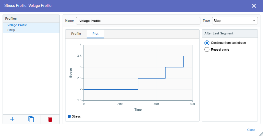
The following is a voltage stress profile example.
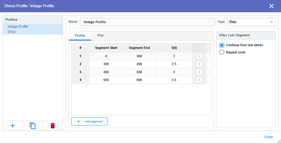
Click on the Plot tab to visualize the profile.
Example 2: Dataset with Time Varying Stress
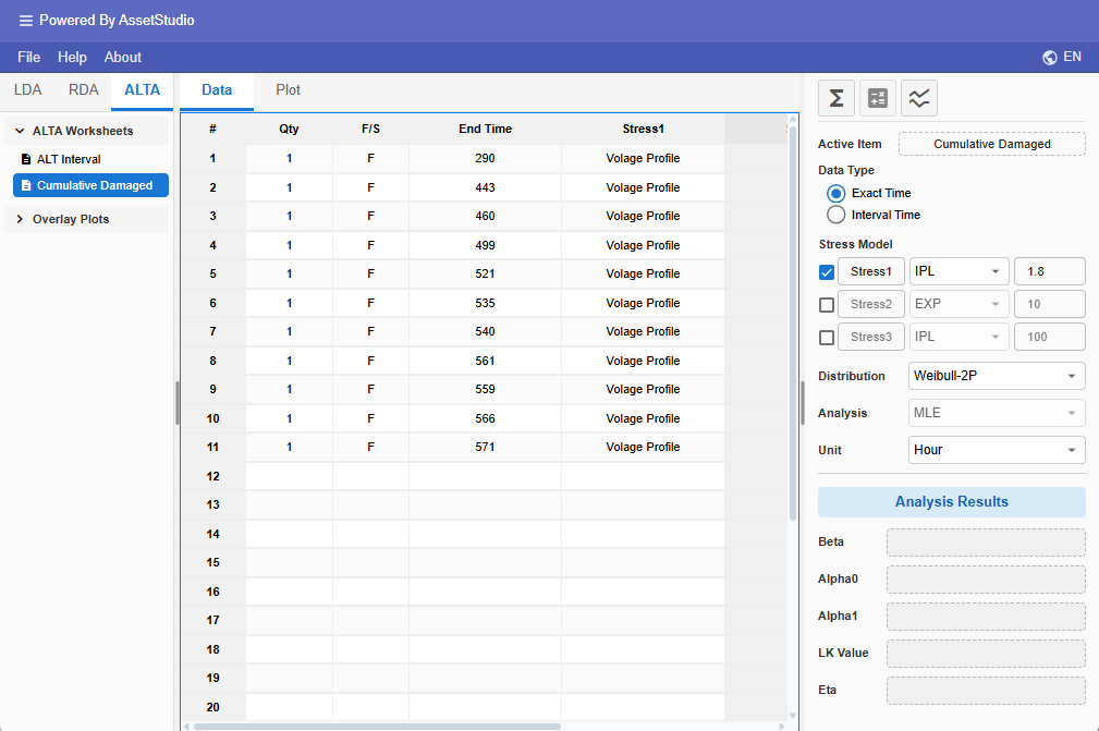
Calculate Parameters
In the main panel, enable one or more stresses and choose a life-stress model for each: Arrhenius, EXP or IPL. Enter the use-level stress used for extrapolation.
Select the life distribution (Weibull-2P, Lognormal or Exponential). Analysis uses MLE.
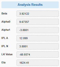
Click on the Analysis icon to calculate the parameters.
The Beta value is the Weibull shape parameter.
The Alpha values are the parameters of the Life-Stress-Relationship model.
Eta value is calculated at use-level stress (1.8 volt in Example 2).
Plots
The following shows the plot for Example 1 (Single Stress).
Once the model parameters are calculated, click on the Plot tab to view the various plots. The default plot type is the Probability plot. You can access the other plots through the Plot Type dropdown list.
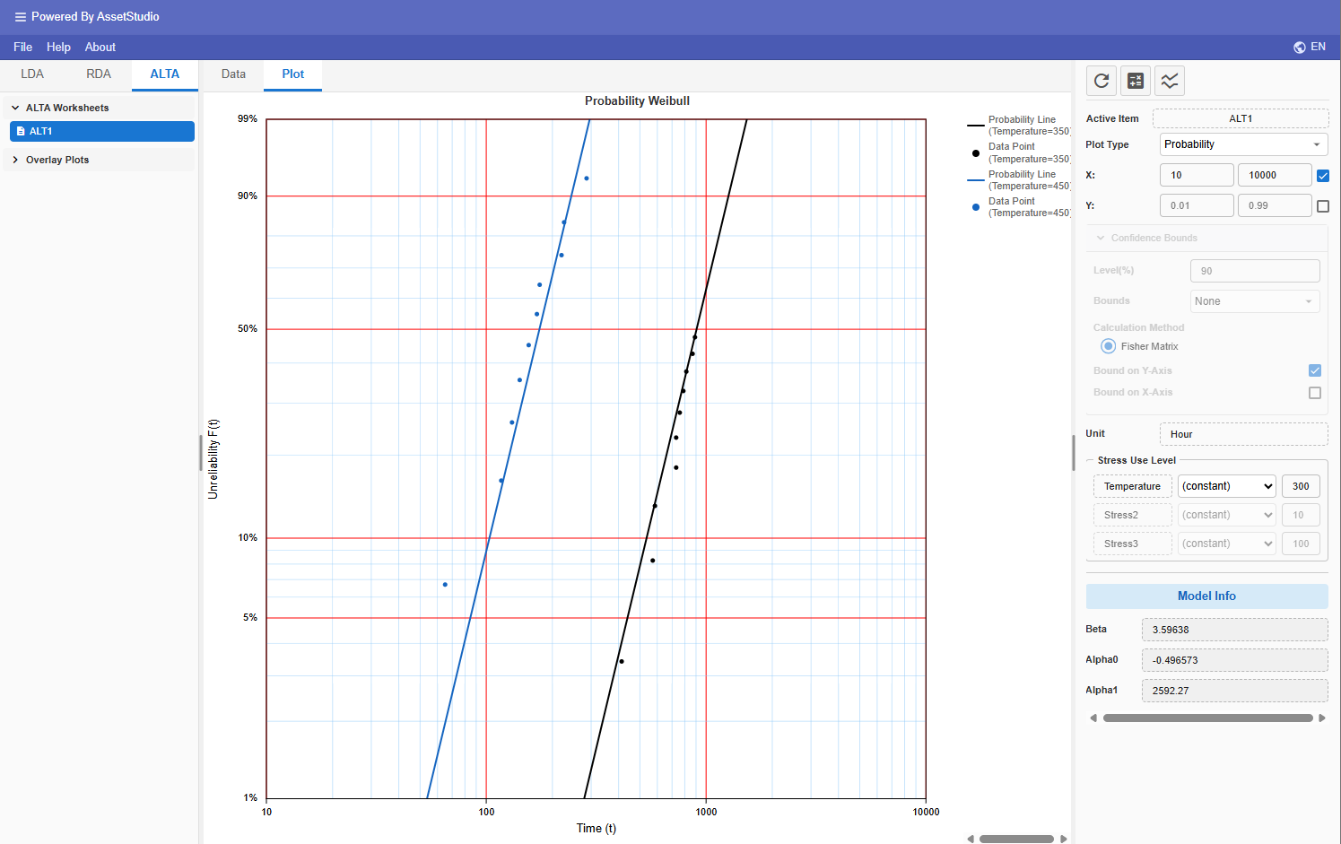
Available plots are:
- Probability Plot
- Use Level Probability Plot
- Reliability vs Time
- Unreliability vs Time (Cumulative Density Function)
- PDF (Probability Density Function)
- Failure Rate vs Time
- Acceleration Factor vs Stress
- Life vs Stress
For Acceleration Factor vs Stress and Life vs Stress, choose which enabled stress varies. Set use-level values in Stress Use Level.
Calculator
Click on the Calculator icon at the top of the main panel.
This tool allows you to query commonly requested reliability results based on your analysis together with required inputs.
| Matrix | Results (at use level) | Required Input |
|---|---|---|
| Reliability | Probability of Success at mission time, T | Time T |
| Unreliability | Probability of Failure at mission time, T | Time T |
| Conditional Reliability | Probability of Success for a mission time t, given start time (current age) T. | Start Time T, and Additional Time t |
| Conditional Unreliability | Probability of Failure for a mission time t, given start time (current age) T. | Start Time T, and Additional Time t |
| BX Life | The time by which X% of the population fails. | Percentage failed BX (%) |
| Warranty Life | The time by which a given fraction of the population still survives. | Reliability |
| Failure Rate | Failure rate at mission time T. | Time T |
| Mean Life | Average life of the population. | None |
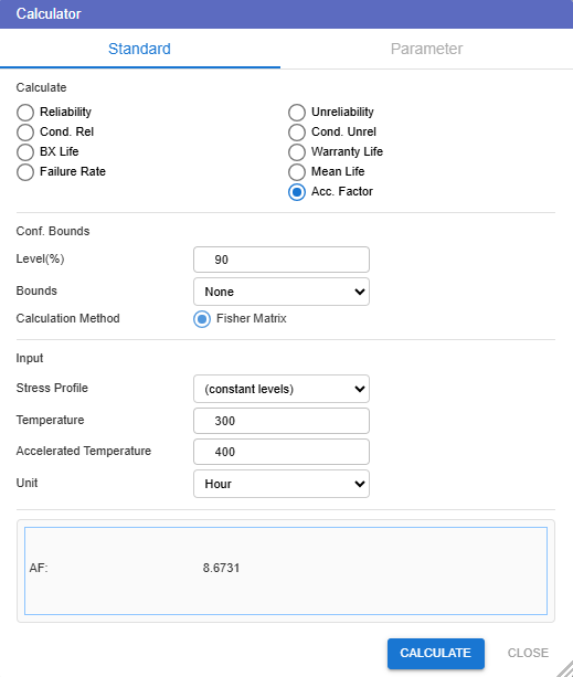
| Acceleration Factor | Ratio of life at use level to accelerated level. | Accelerated level |
Unlike the LDA Calculator, the user needs to provide the use-level stress.
If stress profiles exist, a Stress Profile dropdown appears. Choose a profile, or (constant levels) to evaluate at the use-level stresses.
Time-varying profiles use cumulative exposure (CEM). Mean life is always calculated at constant use stress. Acceleration Factor uses the selected profile as accelerated stress and needs the time at which to evaluate it.
To calculate Acceleration Factor at 450-degree Kelvin with respect to use level (300-degree Kelvin), select Acceleration Factor and enter the accelerated stress.
Overlay Plot
You can compare the plots across different ALTA worksheets using Overlay Plot. This is useful for comparing results from different stress levels, distributions, or life-stress models.
To create an ALTA overlay plot, right-click on Overlay Plots in the ALTA section of the Explorer panel and select Add Overlay Plot.
- Create two or more ALTA worksheets and enter data with different stress levels or settings.
- Analyze each worksheet by clicking the Analysis icon.
- Right-click on Overlay Plots in the Explorer and select Add Overlay Plot.
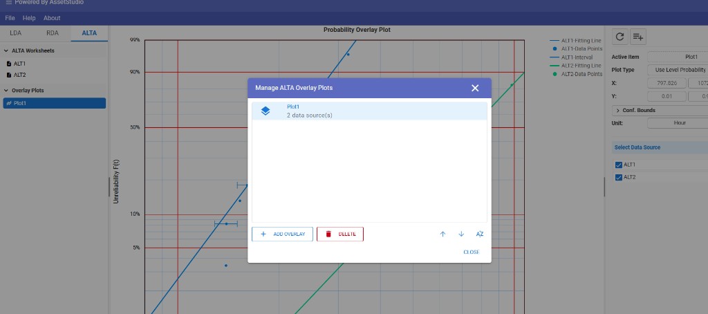
In the Select Data Source dialog, choose the analyzed worksheets you want to overlay, then click OK.
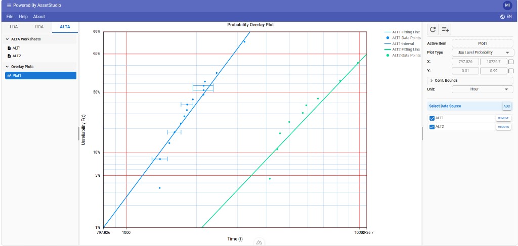
The overlay plot appears in the Plot tab. You can change the plot type, adjust the axis scales, and add confidence bounds using the settings in the main panel.